Creating a Vectorized Convolution layer in NumPy

The code for this project can be found at this link

The Story

Recently I had a class exercise that required creating the convolutional layer used in a convolutional neural network (CNN). The goal was to implement this from scratch, so only basic tools were available to us such as Python and NumPy. When I was trying to figure out how to do this, I did not find any good resource that put the following information together all in one place. I hope that by reading this post you gain a better understanding of the inner workings of a CNN.

For my implementation I decided to go with a vectorized approach as much as possible because this would increase the efficiency of the computations performed on the CPU. I discovered a very helpful resource for performing vectorized matrix operations while also saving a lot of the headache. The links there and basic notes are enough to get you familiar with the np.einsum function. This function may appear daunting at first, but once you start to understand the basics you quickly see how truly powerful NumPy can be.

The convolution layer

Before reviewing the code, you need a little background on what a convolutional layer does under normal operation.

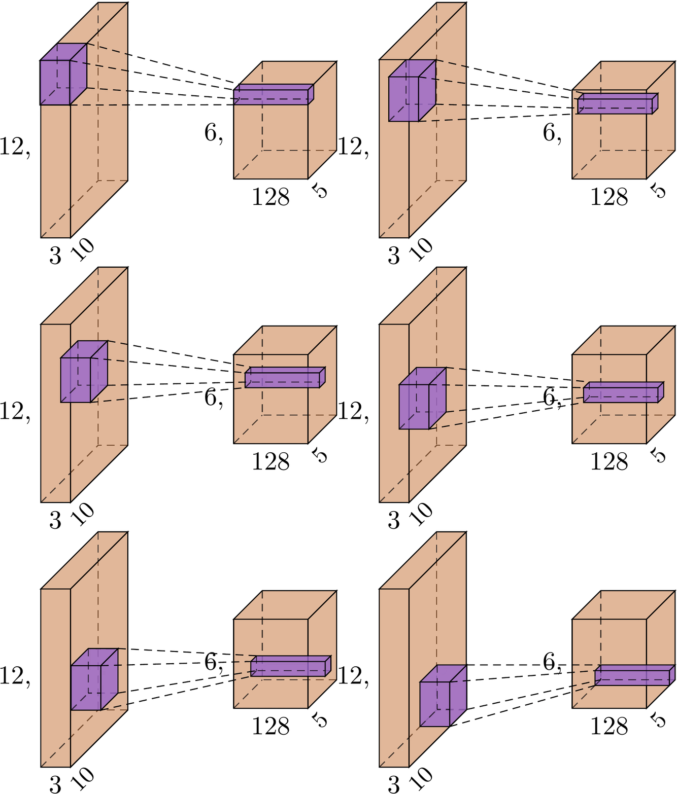
stride=2, kernel_size=2, padding=0, num_filters=128

Here we can see a visual representation of the convolution operation. The convolution layer takes in an input of (channel, height, width) and after convolution returns a matrix of size (num_filters, height’, width’). The act of convolution is using a set of of weights (kernels), num_filters in this case, to extract some features from its input. This happens by the layer “sliding around” its kernels around the input, mapping it to the output tensor. By choosing a stride of two, we are choosing to move the kernels two indices at a time when “sliding” which produces the size reduction you see in the image.

You can more directly control the size of the outputs by adding a padding to the input when performing convolution.

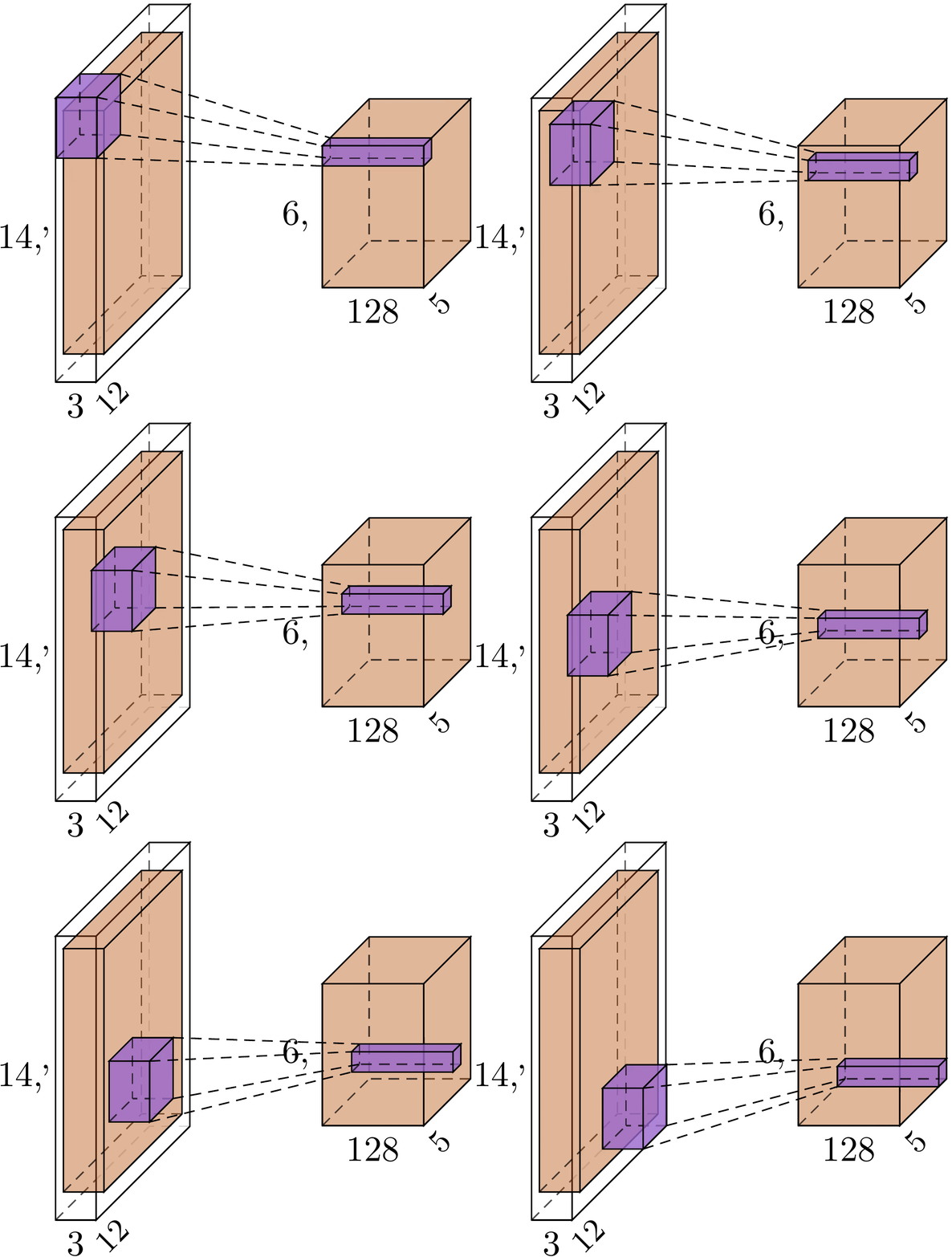
stride=2, kernel_size=3, padding=1, num_filters=128

Here we can see by adding a padding of 1, we add a “buffer” around each edge of the input image. We choose this buffer to be filled with a constant value of zero. This has the effect of allowing the kernel to “look over” the edge of the image, and in turn increases the size of the output image.

One other thing, is that when actually performing training of your CNN you will almost certainly need to pass a batch of images to your model. This allows for more efficient computation and smooths the layer’s gradient when performing gradient descent. To handle this in our layer, we add a dimension to the mentioned inputs. Specifically, instead of handling an image at a time as (C, H, W) we now use (B, C, H, W) where B represents the batch.

Our Approach

Now we can start discussing the actual approach. Here is how we generate the “sliding windows” over the input images.

def getWindows(input, output_size, kernel_size, padding=0, stride=1, dilate=0):
    working_input = input
    working_pad = padding
    # dilate the input if necessary
    if dilate != 0:
        working_input = np.insert(working_input, range(1, input.shape[2]), 0, axis=2)
        working_input = np.insert(working_input, range(1, input.shape[3]), 0, axis=3)

    # pad the input if necessary
    if working_pad != 0: 
        working_input = np.pad(working_input, pad_width=((0,), (0,), (working_pad,), (working_pad,)), mode='constant', constant_values=(0.,))

    in_b, in_c, out_h, out_w = output_size
    out_b, out_c, _, _ = input.shape
    batch_str, channel_str, kern_h_str, kern_w_str = working_input.strides

    return np.lib.stride_tricks.as_strided(
        working_input,
        (out_b, out_c, out_h, out_w, kernel_size, kernel_size),
        (batch_str, channel_str, stride * kern_h_str, stride * kern_w_str, kern_h_str, kern_w_str)
    )

This beautiful piece of code creates the sliding windows over the input images in-memory due to using as_strided. This function tells NumPy how to “walk-memory” in order to create an alternate view of the underlying data. This function works great with our vectorized approach, as all the data remains in a vector.

The getWindows function takes in an input of (B, C, H, W) and outputs of size (B, C, H', W', K, L) where K and L are the kernel height and width respectively. In our case, our kernel is square. So our K and L values will always match, but this notation is important later.

In the forward pass, (H', W') is the output height/width of this layer as determined by the formula:

[(x − kernel_size + (2 * padding)) / stride] + 1

In the backward pass you need to pass back a dx the same size as the x input used in the forward pass, so just copy its size.

The vector (B, C, H, W, K, L) is hard to visualize, but you can think of it as a batch of images where every pixel in the image has an associated KxL window looking at it. This is useful when we combine these windowed inputs with our layer weights.

Dilation is necessary in this function, typically only in the backward pass of the convolution layer. Dilating is useful here when the forward pass uses a convolution stride greater than 1. If that stride results in the output matrix being smaller than the input, then in the backwards pass we need to dilate our gradient to increase its size to match the input matrix. A more detailed explanation with some math is described here.

All the code mentioned in this post is available at this Github Repo.

Creating the convolution layer

Now to continue, we need to create our convolution layer. We will create this as a class for portability, with some basic attributes to control its behavior:

class Conv2D:
    def __init__(self, in_channels, out_channels, kernel_size=3, stride=1, padding=0):
        # number of channels of the input data
        self.in_channels = in_channels
        # number of channels of the output (# filters applied in the layer)
        self.out_channels = out_channels
        # the specified size of the kernel (height & width)
        self.kernel_size = kernel_size
        # the stride of convolution
        self.stride = stride
        # size of padding, to pad zeros to the input with size "padding"
        self.padding = padding

        self.cache = None

        self._init_weights()

    def _init_weights(self):
        self.weight = 1e-3 * np.random.randn(self.out_channels, self.in_channels,  self.kernel_size, self.kernel_size)
        self.bias = np.zeros(self.out_channels)

Forward Pass

We then add the forward pass of the layer

def forward(self, x):
    n, c, h, w = x.shape
    out_h = (h - self.kernel_size + 2 * self.padding) // self.stride + 1
    out_w = (w - self.kernel_size + 2 * self.padding) // self.stride + 1

    windows = getWindows(x, (n, c, out_h, out_w), self.kernel_size, self.padding, self.stride)

    out = np.einsum('bihwkl,oikl->bohw', windows, self.weight)

    # add bias to kernels
    out += self.bias[None, :, None, None]

    self.cache = x, windows
    return out

x: input data of shape (N, C, H, W)

returns: output data of shape (N, self.out_channels, H', W') where H' and W' are determined by the formula mentioned before with getWindows

I’ll review this at a high-level, and then go more into detail. Here, we obtain the vectorized view of the sliding windows over the inputs. We take those windows and then multiply them with our layer weights to extract features from the inputs. Then we add our bias term to our outputs and store our windows in cache for use in the backwards pass of the layer.

The bulk of the work in this forward pass is performed by the NumPy Einsum function. This function makes it possible to perform vectorized operations on matrices, in our case we are multiplying our layer weights with each of the batch images’ sliding windows.

We tell the einsum function to perform this multiplication through use of a convenient equation notation bihwkl,oikl->bohw. If you notice, the first expression in this equation was described before as the output size of the getWindows function. This expression represents the input windows, with each dimension of the input labeled similar to what their dimension represents bihwkl or (batch, input, height, width, kernel_height, kernel_width). The second expression in the equation oikl corresponds to the current weights of the layer which take the shape (num_filter, num_input, kernel_height, kernel_width). By labeling some of these dimensions similarly in the einsum function, we instruct the function to match up these dimensions in the internal calculations. We instruct the function that we want an output of the shape bohw which thanks to our convenient naming represents (batch, num_filter, height, width) which is exactly what we want as output from the layer!

So what’s up? I’ll leave the explanation of the inner workings of einsum to the mentioned very helpful resource. All you need to know, is we somewhat intuitively instructed the computer to multiply the layer weights over a sliding window of the input images. BAM! isnt that simple?

Backward Pass

Now we extend this idea when constructing the backward pass of the layer

def backward(self, dout):
    x, windows = self.cache

    padding = self.kernel_size - 1 if self.padding == 0 else self.padding

    dout_windows = getWindows(dout, x.shape, self.kernel_size, padding=padding, stride=1, dilate=self.stride - 1)
    rot_kern = np.rot90(self.weight, 2, axes=(2, 3))

    db = np.sum(dout, axis=(0, 2, 3))
    dw = np.einsum('bihwkl,bohw->oikl', windows, dout)
    dx = np.einsum('bohwkl,oikl->bihw', dout_windows, rot_kern)

    return db, dw, dx

dout: upstream gradients

returns: dx, dw, and db relative to this module

Here in computing the backwards pass, we find how much each part of our layer contributed to the upstream error. There are many great resources available online which discuss the math which makes this possible. I leave this research as an excercise of the reader and will move on with the “how”, instead of focusing on the “why”.

We start by loading our input windows from the cache for use in our calculations. Similar to creating the windows over the inputs, we now have to create these windows over the upstream gradient, except with a constant stride of 1. We then create a copy of the layer weghts, while rotating the last two dimensions which correspond to the kernel’s height and width. This is necessary in the backward calculations of the layer as it is effectively the opposite of the convolution we performed in forward. Look some into the relationship of convolution and cross-correlation.

Now we can perform the “meat” of the computation by computing how much each part of our layer contributed to the upstream error. Thanks to the partial derivative rule we know that for the bias units, we can just sum the axes of our upstream gradient corresponding to the (batch, height, width) axes which results in a vector sized (num_filters). Next for dW we effectively perform the opposite computation of the forward pass. Instead of combining the weights and the inputs to produce an output, we combine the inputs and the outputs to find the influence the weights had on the outputs. If you look carefully, you can see in this einsum call that we use a similar naming convention as used in the forward pass. For dX we multiply the rotated weights with the windowed upstream gradient to find the influence the input had on the output. This is necessary as this is the value you would pass to preceding layers for their backwards pass.

And thats it!

Well kind of. That’s all the code you need to run the vectorized convolution layer you came here for. Now we show some basic usage/outputs of the layer for demonstration purposes.

Some Examples

We need to define our basic imports and parameters:

import numpy as np

in_channels = 3
out_channels = 128
kernel_size = 3
stride = 2
padding = 1
batch_size = (4, in_channels, 12, 10)  # expected input size
dout_size = (4, out_channels, 6, 5)   # expected to match the size of the layer outputs

np.random.seed(42)  # for reproducibility

Now onto the basic inputs/outputs our layer would expect:

x = np.random.random(batch_size)  # create data for forward pass
dout = np.random.random(dout_size)  # create random data for backward
print('x: ', x.shape)
print('d_out: ', dout.shape)

x:  (4, 3, 12, 10)
d_out:  (4, 128, 6, 5)

Now we need to create an instance of our convolution layer:

conv = Conv2D(in_channels, out_channels, kernel_size, stride, padding)

And finally, we can perform the convolution and backwards operations:

conv_out = conv.forward(x)
db, dw, dx = conv.backward(dout)

print('conv_out: ', conv_out.shape)
print('db: ', db.shape)
print('dw: ', dw.shape)
print('dx: ', dx.shape)

conv_out:  (4, 128, 6, 5)
db:  (128,)
dw:  (128, 3, 3, 3)
dx:  (4, 3, 12, 10)

Thank you all for reading! I know some of this information is dense. I hope after some time reflecting on the information here that you will gain a better understanding of this remarkably powerful deep learning tool.

The code

The code for this project can be found at this link.